AAME 2023 'The Aerial Archaeology Mapping Explorer (AAME) portal', Historic England [website] https://historicengland.org.uk/research/results/aerial-archaeology-mapping-explorer/ [Last accessed: 28 May 2025]
Alberge, D. 2023 'Discovery of up to 25 Mesolithic pits in Bedfordshire astounds archaeologists', The Guardian [website], 3 June 2023. https://www.theguardian.com/science/2023/jul/03/discovery-25-mesolithic-pits-bedfordshire-astounds-archaeologists [Last accessed: 26 March 2025]
Allaby, R., Ware, R., Cribdon, R., Hansford, T., Kinnaird, T., Hamilton, W., Kistler, L., Murgatroyd, P., Bates, R., Fitch, S. and Gaffney, V. 2023 'Pleistocene-Holocene sedaDNA reconstruction of Southern Doggerland reveals early colonization before inundation consistent with northern refugia', 21 September 2023, PREPRINT (Version 1), Research Square. [Last accessed: 11 June 2025] https://doi.org/10.21203/RS.3.RS-3296992/V1
Baldwin, E. and V. Gaffney 2020 'Interim report on the recent discovery of a series of massive pits near the Durrington Walls henge', Unpublished Report for the National Trust, University of Birmingham
Bøtter-Jensen, L., McKeever, S.W. and Wintle, A.G. 2003 Optically Stimulated Luminescence Dosimetry, Amsterdam: Elsevier. https://doi.org/10.1016/B978-0-444-50684-9.X5077-6
Bowden, M., Soutar, S., Field, D. and Barber, M. 2015 The Stonehenge Landscape. Analysing the Stonehenge World Heritage Site, Swindon: Historic England.
Bradley, R. 1998 The Significance of Monuments, London: Routledge.
Bradley, R. 2012 The Idea of Order: The Circular Archetype in Prehistoric Europe, Oxford University Press. https://doi.org/10.1093/oso/9780199608096.001.0001
Ch'ng, E., Gaffney, V. and Hakvoort, G. 2014 'Stigmergy in comparative settlement choice and palaeoenvironment simulation', Complexity 21(3), 59–73. https://doi.org/10.1002/cplx.21616
Chartres, C.J. and Whalley, W.B. 1975 'Evidence for Late Quaternary solution of Chalk at Basingstoke, Hampshire', Proceedings of the Geologists' Association 86(3), 365–72. https://doi.org/10.1016/S0016-7878(75)80027-7
Condit, T. and Keegan, M. 2018 'Aerial investigation and mapping of the Newgrange landscape, Brú na Bóinne, Co. Meath. The Archaeology of the Brú na Bóinne World Heritage Site Interim Report, December 2018, Department of Culture, Heritage and the Gaeltacht', Voices from the Dawn [website]. https://voicesfromthedawn.com/wp-content/sites/newgrange/bru-na-boinne-interim-report_web.pdf [Last accessed: 11 June 2025]
Condit, T. and Keegan, M. 2020. 'A Neolithic ritual landscape revealed: A summary of the principal sites that were identified on the Newgrange floodplain during the drought conditions of summer 2018', OPW – Oidhreacht Éireann/Heritage Ireland [website] https://heritageireland.ie/articles/a-neolithic-ritual-landscape-revealed/ [Last accessed: 11 June 2025]
Cribdon, B., Ware, R., Smith, O., Gaffney, V. and Allaby, R. 2020 'PIA: more accurate taxonomic assignment of Metagenomic Data demonstrated on sedaDNA from the North Sea', Frontiers in Ecology and Evolution 8(84). https://doi.org/10.3389/fevo.2020.00084
Crutchley, S. 2002 'Stonehenge World Heritage Site Mapping Project: Management Report', Aerial Survey Report Series AER/14/2002, Swindon: English Heritage. https://historicengland.org.uk/research/results/reports/6835/StonehengeWorldHeritageSiteMappingProject_ManagementReport [Last accessed: 28 May 2025]
Darvill, T. 1997 'Ever increasing circles: the sacred geographies of Stonehenge and its landscape' in B. Cunliffe and C. Renfrew (eds) Science and Stonehenge, Proceedings of the British Academy 92, 167–202. http://publications.thebritishacademy.ac.uk/pubs/proc/volumes/pba92.html
Davis, S. and Rassmann, K. 2021 'Beyond Newgrange: Brú na Bóinne in the later Neolithic', Proceedings of the Prehistoric Society 87, 189–218. https://doi.org/10.1017/ppr.2021.6
Dietze, M., Kreutzer, S., Fuchs, M. C., Burow, C., Fischer, M. and Schmidt, C. 2013 'A practical guide to the R package Luminescence', Ancient TL 32, 11-18. https://doi.org/10.26034/la.atl.2013.469
Dingwall, K. 2018 'Highway through History – An archaeological journey on the Aberdeen Western Peripheral Route', Edinburgh: Headland Archaeology (UK) Ltd. Còmhdhail Alba/Transport Scotland [website] https://www.transport.gov.scot/media/44074/highway-through-history.pdf [Last accessed: 11 June 2025]
Duller, G.A.T. 2003 'Distinguishing quartz and feldspar in single grain luminescence measurements', Radiation Measurements 37(2), 161-65. https://doi.org/10.1016/S1350-4487(02)00170-1
>
Ellwood, B.B., Tomkin, J.H., Ratcliffe, K.T., Wright, M. and Kafafy, A.M. 2008 'High-resolution magnetic susceptibility and geochemistry for the Cenomanian/Turonian boundary GSSP with correlation to time equivalent core', Palaeogeography, Palaeoclimatology, Palaeoecology 261(1-2), 105–26. https://doi.org/10.1016/j.palaeo.2008.01.005
Everett, R. and Cribdon, B. 2023 'MetaDamage tool: examining post-mortem damage in sedaDNA on a metagenomic scale', Frontiers in Ecology and Evolution 10, 888421, 1-15. https://doi.org/10.3389/fevo.2022.888421
Exon, S., Gaffney, V., Woodward, A. and Yorston, R. 2001 Stonehenge Landscapes: Journeys Through Real–And–Imagined Worlds, Oxford: Archaeopress. [CD published 2000]
Finlay, A., Bates, R., Bensharada, M. and S. Davies 2022 'Applying chemostratigraphic techniques to shallow bore holes: lessons and case studies from Europe's lost frontiers' in V. Gaffney and S. Fitch (eds) Europe's Lost Frontiers Volume 1 – Context and Methodology, Oxford, Archaeopress. 137–153. https://doi.org/10.32028/9781803272689
Gaffney, V., Neubauer, W. and Gaffney, C. 2010 'Stonehenge Hidden Landscapes – Project Design' (submitted to the National Trust and English Heritage), University of Birmingham.
Gaffney, C., Gaffney, V., Neubauer, W., Baldwin, E., Chapman, H., Garwood, P., Moulden, H., Sparrow, T., Bates, R., Löcker, K., Hinterleitner, A., Trinks, I., Nau, E., Zitz, T., Flöry, S., Verhoeven, G. and Doneus, M. 2012 'The Stonehenge Hidden Landscapes Project', Archaeological Prospection 19(2), 147–55. https://doi.org/10.1002/arp.1422
Gaffney, V., Fitch, S., Ramsey, E., Yorston, R., Ch'ng. E., Baldwin, E., Bates, R., Gaffney, C., Ruggles, C., Sparrow, T., McMillan, A., Cowley, D., Fraser, S., Murray, C, Murray, H., Hopla, E. and Howard., A 2013 'Time and a place: a lunisolar 'time-reckoner' from 8th millennium BC Scotland', Internet Archaeology 34. http://dx.doi.org/10.11141/ia.34.1
Gaffney, V., Neubauer, W., Garwood, P., Gaffney, C., Löcker, K., Bates, R., De Smedt, P., Baldwin, E., Chapman, H., Hinterleitner, A., Wallner, M., Nau, E., Filzwieser, R., Kainz, J., Trausmuth, T., Schneidhofer, P., Zotti, G., Lugmayer, A., Trinks, I. and Corkum, A. 2018 'Durrington Walls and the Stonehenge Hidden Landscape Project 2010-2016', Archaeological Prospection 25(3), 1–15. https://doi.org/10.1002/arp.1707
Gaffney, V., Baldwin, E., Bates, M., Bates, R., Gaffney, C., Hamilton, D., Kinnaird, T., Neubauer, W., Yorston, R., Allaby, R., Chapman, H., Garwood, P., Löcker, K., Hinterleitner, A., Sparrow, T., Trinks, I., Wallner, M. and Leivers, M. 2020 'A massive, Late Neolithic pit structure associated with Durrington Walls Henge', Internet Archaeology 55. https://doi.org/10.11141/ia.55.4
Gaffney, V., Fitch, S., Bates, M., Ware, R.L., Kinnaird, T., Gearey, B., Hill, T., Telford, R., Batt, C., Stern, B., Whittaker, J., Davies, S., Ben Sharada, M., Everett, R., Cribdon, R., Kistler, L., Harris, S.,Kearney, K., Walker, J., Muru, M., Hamilton, D., Law, M. and Finlay, A. 2020 'Multi-Proxy Characterisation of the Storegga Tsunami and Its Impact on the Early Holocene Landscapes of the Southern North Sea', Geosciences 10(7), 270. https://doi.org/10.3390/geosciences10070270
Gaffney, V., Gaffney C. and Walker, J. 2023 'Extensive Mesolithic discovery in Bedfordshire shows the importance of pits for understanding early Britain', The Conversation [website] https://doi.org/10.64628/AB.hm36mnpd5
Grassé, P.P. 1959 'La reconstruction du nid et les coordinations interindividuelles chez Bellicositermes natalensis et Cubitermes sp. la théorie de la stigmergie: Essai d'interprétation du comportement des termites constructeurs', Insectes Sociaux 6(1), 41–80. https://doi.org/10.1007/BF02223791
Guérin, G., Mercier, N., & Adamiec, G. 2011 'Dose-rate conversion factors: update', Ancient TL 29(1), 5–8. https://doi.org/10.26034/la.atl.2011.443
Guérin, G., Christophe, C., Philippe, A., Murray, A. S., Thomsen, K. J., Tribolo, C., Urbanova, P., Jain, M., Guibert, P., Mercier, N., Kreutzer, S. and Lahaye, C. 2017 'Absorbed dose, equivalent dose, measured dose rates, and implications for OSL age estimates: introducing the Average Dose Model', Quaternary Geochronology 41, 163–73. https://doi.org/10.1016/j.quageo.2017.04.002
Guérin, G., Mercier, N., Nathan R., Adamiec, G., and Lefrais, Y. 2012 'On the use of the infinite matrix assumption and associated concepts: a critical review', Radiation Measurements 47(9), 778–785. https://doi.org/10.1016/j.radmeas.2012.04.004
Helbing, D., Keltsch, J. and Molnar, P. 1997a 'Modelling the evolution of human trail systems', Nature 388, 47–50. https://doi.org/10.1038/40353
Helbing, D., Schweitzer, F., Keltsch, J. and Molna, P. 1997b 'Active walker model for the formation of human and animal trail systems', Physical Review E 56, 2527–39. http://link.aps.org/doi/10.1103/PhysRevE.56.2527
Historic England 2024 'The National Heritage List for England (NHLE) – register of all nationally protected historic buildings and sites in England', Historic England [website] https://historicengland.org.uk/listing/the-list/ [Last accessed: 28 May 2025]
Hopson, P., Farrant, A., Newell, A., Marks, R.J., Booth, K., Bateson, L., Woods, M., Wilkinson, I., Brayson, J. and Evans, D. 2006 'Geology of the Salisbury Sheet Area: report on the geology of Sheet 298 Salisbury and its adjacent area. A compilation of the results of the survey in spring and autumn 2003 and from the River Bourne survey of 1999', Internal Report IR/06/011 (unpublished), Nottingham: British Geological Survey. https://nora.nerc.ac.uk/id/eprint/7175
Jarvis, I. and Jarvis, K. E. 1992 'Inductively coupled plasma-atomic emission spectrometry in exploration geochemistry', Journal of Geochemical Exploration 44(1-3), 139-200. https://doi.org/10.1016/0375-6742(92)90050-I
Jarvis, I. and Jarvis, K.E. 1992b 'Plasma spectrometry in the earth sciences: techniques, applications and future trends', Chemical Geology 95, 1–33. https://doi.org/10.1016/0009-2541(92)90041-3
Jeffrey, Z.E., Penn, S., Giles, P.G. and Hastewell, L. 2020 'Identification, investigation and classification of surface depressions and chalk dissolution features using integrated LiDAR and geophysical methods', Quarterly Journal of Engineering Geology and Hydrogeology 53, 620–44. https://doi.org/10.1144/qjegh2019-098
John, B. 2020 'Durrington super-circuit: an hypothesis full of holes', Stonehenge and the Ice Age [website] https://brian-mountainman.blogspot.com/2020/06/durrington-super-circuit-hypothesis.html [Last accessed: 4 December 2024]
Kinnaird, T.C., Abellán Santisteban, J., Brandolini, F., Carlton, R., Carrer, F., Civantos, J.M.M., Duggan, M., Holcomb, J.A., Lekakis, S., Ramos Rodríguez, B., Salazar Ortiz, N., Sánchez-Pardo, J.C., Sevara, C., Snyder, J.R., Shillito, L.-M., Silva Sanchez, N., Srivastava, A., Turner, A. and Turner, S. 2025 'Unearthing the histories of agrarian landscapes: a research framework for terraces as sustainable environments', Geoarchaeology 40, e70004. https://doi.org/10.1002/gea.70004
Kinnaird, T.C., Bolòs, J., Turner, A. and Turner, S. 2017a 'Optically-stimulated luminescence profiling and dating of historic agricultural terraces in Catalonia (Spain)', Journal of Archaeological Science 78, 66–77. https://doi.org/10.1016/j.jas.2016.11.003
Kinnaird, T.C., Dawson, T., Sanderson, D.C.W., Hamilton, D., Cresswell, A. and Rennel, R., 2017b. 'Chronostratigraphy of an eroding complex Atlantic round house, Baile Sear, Scotland', Journal of Coastal and Island Archaeology 14(1), 46–60. https://doi.org/10.1080/15564894.2017.1368744
Kircher, M., Sawyer, S., & Meyer, M. 2012 'Double indexing overcomes inaccuracies in multiplex sequencing on the Illumina platform', Nucleic Acids Research 40(1). https://doi.org/10.1093/nar/gkr771
Kolb, T., Tudyka, K., Kadereit, A., Lomax, J., Poreba, G., Zander, A., Zipf, L. and Fuchs, M. 2021 'Data for “The µDose-system: determination of environmental dose rates by combined alpha and beta counting – performance tests and practical experiences”', JLUpub [dataset], https://doi.org/10.22029/jlupub-39
Kolb, T., Tudyka, K., Kadereit, A., Lomax, J., Poreba, G., Zander, A., Zipf, L. and Fuchs, M., 2022. 'The µDose system: determination of environmental dose rates by combined alpha and beta counting – performance tests and practical experiences', Geochronology 4, 1–31. https://doi.org/10.5194/gchron-4-1-2022
Kreutzer, S., Burow, C., Dietze, M., Fuchs, M.C., Schmidt, C., Fischer, M., Friedrich, J., Mercier, N., Smedley, R., Christophe, C., Zink, A., Durcan, J.A., King, G.E., Philippe, A., Guérin, G., Riedesel, S., Autzen, M., Guibert, P., Mittelstraß, D., Gray, H.J. and Galharret, J-M. 2024 Luminescence: Comprehensive Luminescence Dating Data Analysis https://zenodo.org/records/6345291 [Last accessed: 12 June 2025]
Leivers, M. 2021 'The Army Basing Programme, Stonehenge and the emergence of the Sacred Landscape of Wessex', Internet Archaeology 56. https://doi.org/10.11141/ia.56.2
Leivers, M., Thompson, S., Valdez-Tullett, A. and Wakeham, G. 2020 'Larkhill Service Family Accommodation, Larkhill, Wiltshire Post-excavation Assessment Report', Unpublished report: Wessex Archaeology.
Luke, M. and Kozimiński, M. 2023 'Chapter 4 - Late Mesolithic to Roman land-use at site HRN3486' in M. Luke and D. Shotliff (eds) Late Mesolithic to Early Anglo-Saxon Land-use at Houghton Regis North, Bedfordshire: Sites HRN3205, HRN3455/6/7, HRN3486 and Woodside Link, Albion Archaeology Monograph 11, Bedford: Albion Archaeology. 79–124.
Mejdahl, V. 1979 'Thermoluminescence dating: Beta-dose attenuation in quartz grains', Archeometry 29(1), 61–72. https://doi.org/10.1111/j.1475-4754.1979.tb00241.x
Meyer, M., and Kircher, M. 2010 'Illumina sequencing library preparation for highly multiplexed target capture and sequencing', Cold Spring Harbor Protocols 2010(6), pdb.prot5448. https://doi.org/10.1101/pdb.prot5448
Morris, S. 2024 'Two newly discovered stone circles on Dartmoor boost 'sacred arc' theory', The Guardian [website], 15 November 2024. https://www.theguardian.com/science/2024/nov/15/two-newly-discovered-stone-circles-dartmoor-sacred-arc-theory. [Last accessed: 11 September 2025]
Munyikwa, K., Kinnaird, T.C., and Sanderson, D.C.W. 2021 'The potential of portable luminescence readers in geomorphological investigations: a review', Earth Surface Processes and Landforms 46(1), 131–50. https://doi.org/10.1002/esp.4975
Murray, A. S. and Wintle, A. G. 2000 'Luminescence dating of quartz using an improved single-aliquot regenerative-dose protocol', Radiation Measurements 32(1), 57–73. https://doi.org/10.1016/S1350-4487(99)00253-X
Olesik, J.W. 1991 'Elemental analysis using ICP-OES and ICP/MS', Analytical Chemistry 63, 12A-21A. https://doi.org/10.1021/ac00001a711
Parker Pearson, M. and Ramilisonina, 1998 'Stonehenge for the ancestors: the stones pass on the message', Antiquity 72(276), 308–26. https://doi.org/10.1017/S0003598X00086592
Pollard, J. 1995 'Inscribing space: formal deposition at the Later Neolithic monument of Woodhenge, Wiltshire', Proceedings of the Prehistoric Society 61, 137-56. https://doi.org/10.1017/S0079497X00003066
Prescott, J.R. and Hutton, J.T. 1994 'Cosmic ray contributions to dose-rates for luminescence and ESR dating: large depths and long-term time variations', Radiation Measurements 23, 497-500. http://dx.doi.org/10.1016/1350-4487(94)90086-8
Rohland, N. and Reich, D. 2012 'Cost-Effective, High-Throughput DNA Sequencing Libraries for Multiplexed Target Capture', Genome Research 22(5), 939-946. https://doi.org/10.1101/gr.128124.111
Royal Commission On Historical Monuments (England) (RCHME) 1979 Stonehenge and its Environs: Monuments and Land Use, Edinburgh: Edinburgh University Press.
Ruggles, C. and Chadburn, A. 2024 'Missing data', Cosmovisiones/Cosmovisões 5, 99-109. https://doi.org/10.24215/26840162e007
Schmidt, A. and Crabb, N. 2017 'Larkhill SFA Haul Road, Larkhill, Wiltshire - Detailed Gradiometer Survey Report', Unpublished report: Wessex Archaeology.
De Smedt, P., Garwood, P., Chapman, H., Deforce, K., De Grave, J., Hanssens, D. and Vandenberghe. D. 2022 'Novel insights into prehistoric land use at Stonehenge by combining electromagnetic and invasive methods with a semi-automated interpretation scheme', Journal of Archaeological Science 143. https://doi.org/10.1016/j.jas.2022.105557
>
Sperling, C.H.B., Goudie, A.S., Stoddart, D.R. and Poole, G.G. 1977 'Dolines of the Dorset Chalklands and other areas in southern Britain', Transactions of the Institute of British Geographers 2(2), 205-23. https://doi.org/10.2307/621858
Thompson, S. and Powell, A.B. 2018 Along Prehistoric Lines: Neolithic, Iron Age and Romano-British activity at the former MOD Headquarters, Durrington, Wiltshire, Oxford: Oxbow Books.
Thorez, J., Bullock, P., Catt, J.A. and Weir, A.H. 1971 'The petrography and origin of deposits filling solution pipes in the Chalk near South Mimms, Hertfordshire', Geological Magazine 108(5), 413-23. https://doi.org/10.1017/S0016756800056454
Tilley C. 1994 A Phenomenology of Landscape: places, paths, and monuments, Oxford: Berg.
Tudyka, K., Mi?osz, S., Adamiec, G., Bluszcz, A., Poreba, G., Paszkowski, L. and Kolarczyk, A. 2018 'μDose: A compact system for environmental radioactivity and dose rate measurement', Radiation Measurements 118, 8–13. https://doi.org/10.1016/j.radmeas.2018.07.016
Turner, S., Kinnaird, T., Varinlioglu, G., Emre Şerifoğlu, T., Koparal, E., Demirciler, V.
, Athanasoulis, D., Ødegård, K., Crow, J., Jackson, M., Bolòs, J., Sánchez-Pardo, J.C., Carrer, F., Sanderson, D. and Turner, A. 2021 'Agricultural terraces in the Mediterranean: medieval intensification revealed by OSL profiling and dating', Antiquity 95(381), 773–90. https://doi.org/10.15184/aqy.2020.187
Tyler, G. and Jobin Yvon, S. 1995 'ICP-OES, ICP-MS and AAS Techniques Compared', ICP Optical Emission Spectroscopy Technical Note 5, New Jersey: Edison.
Urmston, B. 2014 'Army Rebasing: Larkhill East Site, Salisbury, Wiltshire – Detailed Gradiometer Survey Report', Unpublished report: Wessex Archaeology. https://doi.org/10.5284/1048789
Waltham, T., Bell, F. and Culshaw, M. 2005 Sinkholes and Subsidence, Karst and Cavernous Rocks in Engineering and Construction, Heidelberg: Springer Praxis Publishing. https://doi.org/10.1007/b138363
Wolframm-Murray, Y. 2024 'Archaeological strip, map and sample at Parcel 1, Linmere Phase 1 Houghton Regis North 1 Central Bedfordshire Report No. 24/009', Unpublished report, Northampton: Museum of London Archaeology (Mola).
Woodward A.B. and Woodward P.J. 1996 'The Topography of some Barrow Cemeteries in Bronze Age Wessex', Proceedings of the Prehistoric Society 62, 275-291. https://doi.org/10.1017/S0079497X00002814
Worley, F., Madgwick, R., Pelling, R., Marshall, P., Evans, J.A., Lamb, A.L., López-Dóriga, I.L., Bronk Ramsey, C., Dunbar, E., Reimer, P., Vallender, J. and Roberts, D. 2019 'Understanding Middle Neolithic food and farming in and around the Stonehenge World Heritage Site: An integrated approach', Journal of Archaeological Science: Reports 26, 101838. https://doi.org/10.1016/j.jasrep.2019.05.003
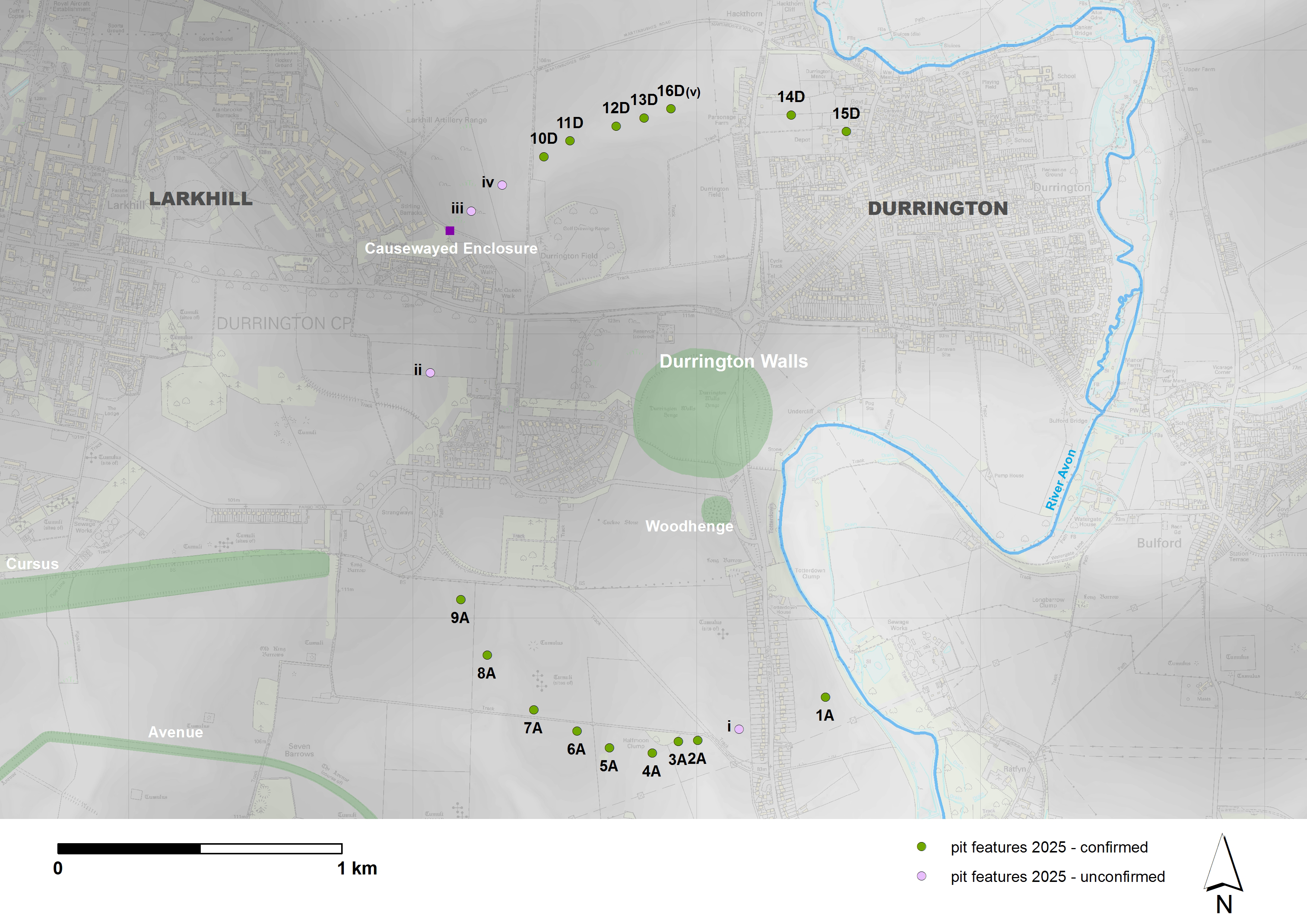
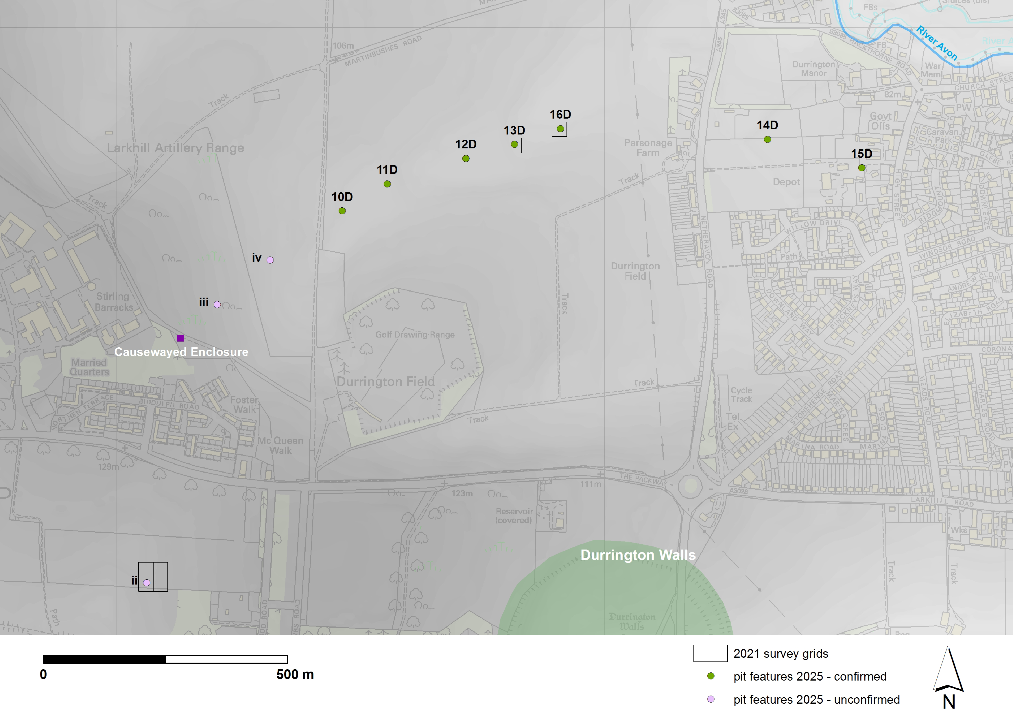
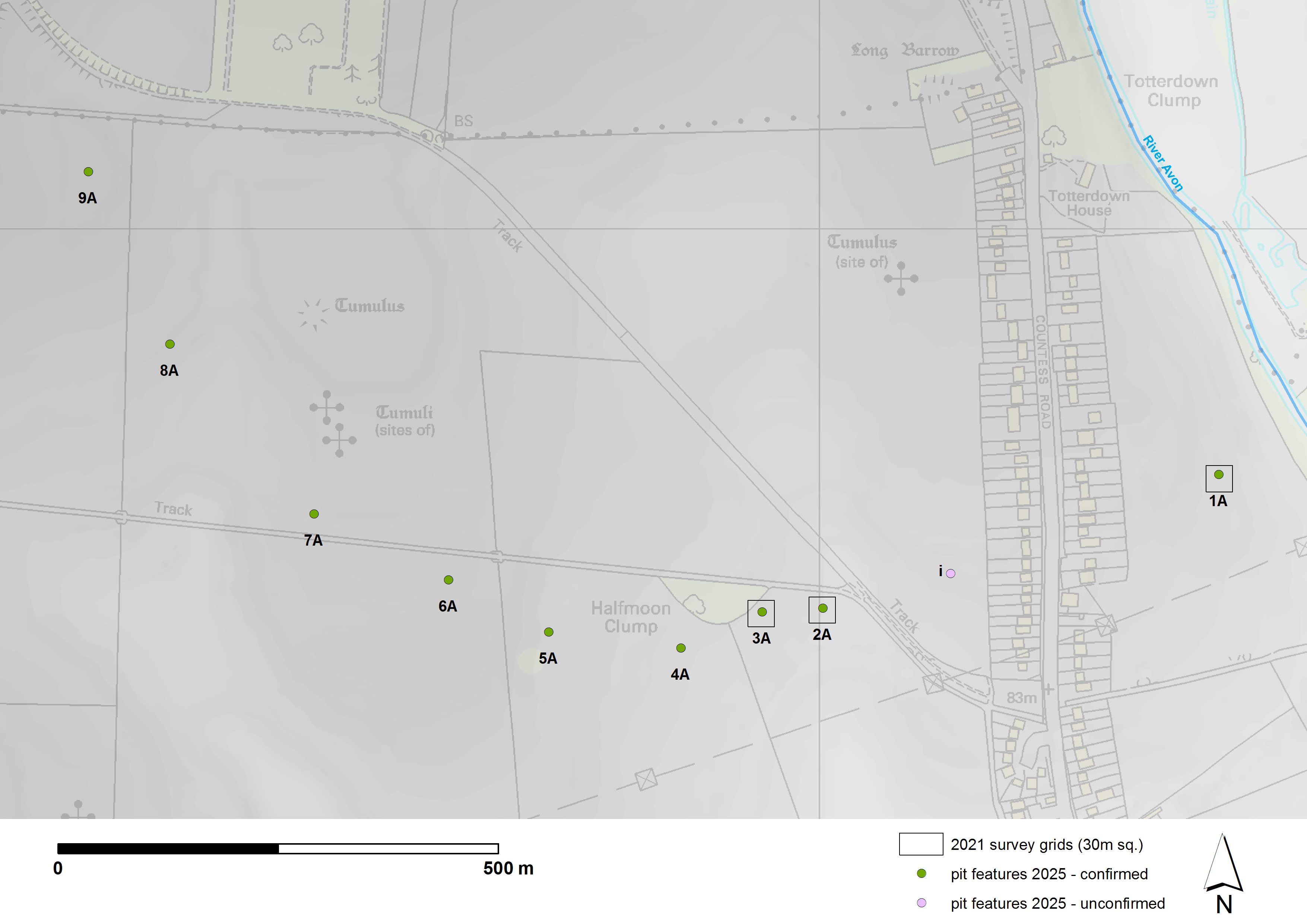
 Home Summary